AeroShieldMimic Class
- class automationshield.AeroShieldMimic(discretisation: str | None = None)[source]
Bases:
StateSpaceShield,AeroShieldState-space model of the AeroShield. Simulates the behaviour of an Aeroshield device through its range of angles. The system is identified through the following set of differential equations
\[\begin{split}\ddot{\theta} &= \frac{k \cdot F}{m \cdot r} - \frac{g}{r} \sin{\theta} - \frac{b \cdot \dot{\theta}}{m \cdot r} \\ \dot{\theta} &= \dot{\theta} \\ \dot{F}_k &= d \cdot \left(u_{k-1} - F_{k-1}\right)\end{split}\]Here, \(k \cdot F\) is the fan thrust, with \(k\) a constant and \(F\) an approximation of the fan speed. The fan speed is modelled as a delay between the requested input and the effective fan speed. The value of \(d\) was obtained through frequency analysis.
The system of equations is converted to a state-space system to work with the
StateSpaceShield. Inputs and outputs are identical to the physical shield, the state vector is\[\begin{split}x = \begin{bmatrix} \dot{\theta} \\ \theta \\ F \end{bmatrix}\end{split}\]For the matrices, refer to the methods in which they are defined.
The state-space system is linearised each control loop at its current position, such that the behaviour more closely resembles real life. For this, a second-degree polynomial that models the required input to hold the pendulum at a given angle was obtained experimentally. This polynomial is given in
AeroShieldMimic.equilibrium.- Parameters:
discretisation (str) – Discretisation method to use, defaults to the default of
StateSpaceShield.
- b = 0.0007
Friction coefficient.
- m = 0.006
Pendulum mass.
- g = 9.81
Gravitational acceleration.
- r = 0.125
Pendulum length.
- k = 0.00165
Fan thrust multiplier.
- d = 12
Fan speed delay constant.
- equilibrium: poly1d = poly1d([11.94686247, 29.28852909, 1.04011991])
Second-degree polynomial returning the required steady-state input as a function of the sine of the pendulum angle. The figure shows the input required to keep the pendulum at a given angle, i.e. compensate for its own weight.
(
Source code,png,hires.png,pdf)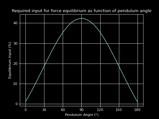
- calculate_a(state: ndarray[tuple[int, ...], dtype[float64]]) ndarray[tuple[int, ...], dtype[float64]][source]
Calculate matrix A:
\[\begin{split}A = \begin{bmatrix} -\frac{b}{m \cdot r} & - \frac{g}{r} \cos{\theta} & \frac{k}{m \cdot r} \\ 1 & 0 & 0 \\ 0 & 0 & -12 \\ \end{bmatrix}\end{split}\]where \(\theta\) is a state variable.
- calculate_b(state: ndarray[tuple[int, ...], dtype[float64]]) ndarray[tuple[int, ...], dtype[float64]][source]
Calculate matrix B:
\[\begin{split}B = \begin{bmatrix} 0 \\ 0 \\ 12 \end{bmatrix}\end{split}\]
- calculate_c(state: ndarray[tuple[int, ...], dtype[float64]]) ndarray[tuple[int, ...], dtype[float64]][source]
Calculate matrix C:
\[C = \begin{bmatrix} 0 & 1 & 0 \end{bmatrix}\]
- calculate_d(state: ndarray[tuple[int, ...], dtype[float64]]) ndarray[tuple[int, ...], dtype[float64]][source]
Calculate matrix D:
\[D = \begin{bmatrix} 0 \end{bmatrix}\]
- get_equilibrium_point(state: ndarray[tuple[int, ...], dtype[float64]]) tuple[ndarray[tuple[int, ...], dtype[float64]], float][source]
Calculate equilibrium input and state at the current pendulum angle \(\theta\). The equilibrium state is defined as
\[\begin{split}x_{e, k} = \begin{bmatrix} \dot{\theta}_{e, k} \\ \theta_{e, k} \\ F_{e, k} \end{bmatrix} = \begin{bmatrix} 0 \\ \theta_k \\ u_{e,k} \end{bmatrix}\end{split}\]